Contributions

Selected accomplishments

Software platform

The first reduced-order modelling library combining comprehensiveness, modularity, and high-level API

GridapROMs.jl is, as far as I know, the first reduced-order modelling library to combine this much breadth with an interface that is genuinely easy to use. This was also a major design objective of GridapROMs.jl's parent library, Gridap.jl, and which I extended to tackle parameterised equations in a reduced-order context. It supports POD, Tucker, tensor-train, interpolation, and localised subspace strategies, all exposed through the same high-level API, so moving between them is a matter of changing how the reduced space is built, not rewriting the surrounding code. That combination of comprehensiveness and modularity is what makes it practical on real problems: reduced-order algorithms built with the library have achieved speedups several thousand times over full-order simulations.
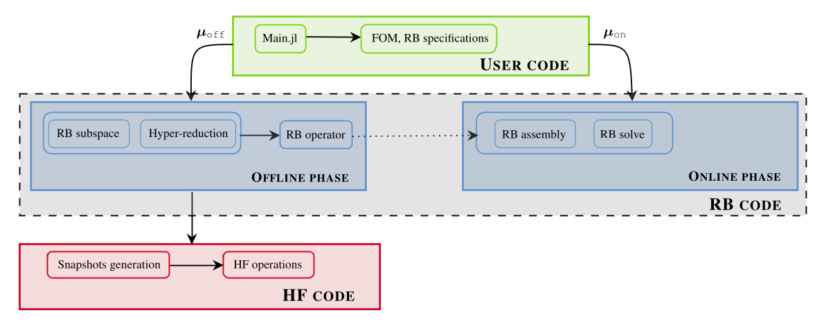
GridapROMs.jl architecture diagram

Overview of GridapROMs.jl's structure. The user defines reduced-order models which rely on a layer of lower-level high-fidelity operations, ranging from integration to solution of the parameterised systems of interest.
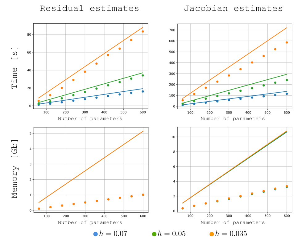
Time and memory cost of parametric assembly

Wall time and memory for assembling a parametric residual/Jacobian, GridapROMs.jl (dots) vs. a naive per-parameter loop (lines), across three mesh resolutions (h) and number of parameters.
Geometric flexibility

Reduced order models built for changing geometries

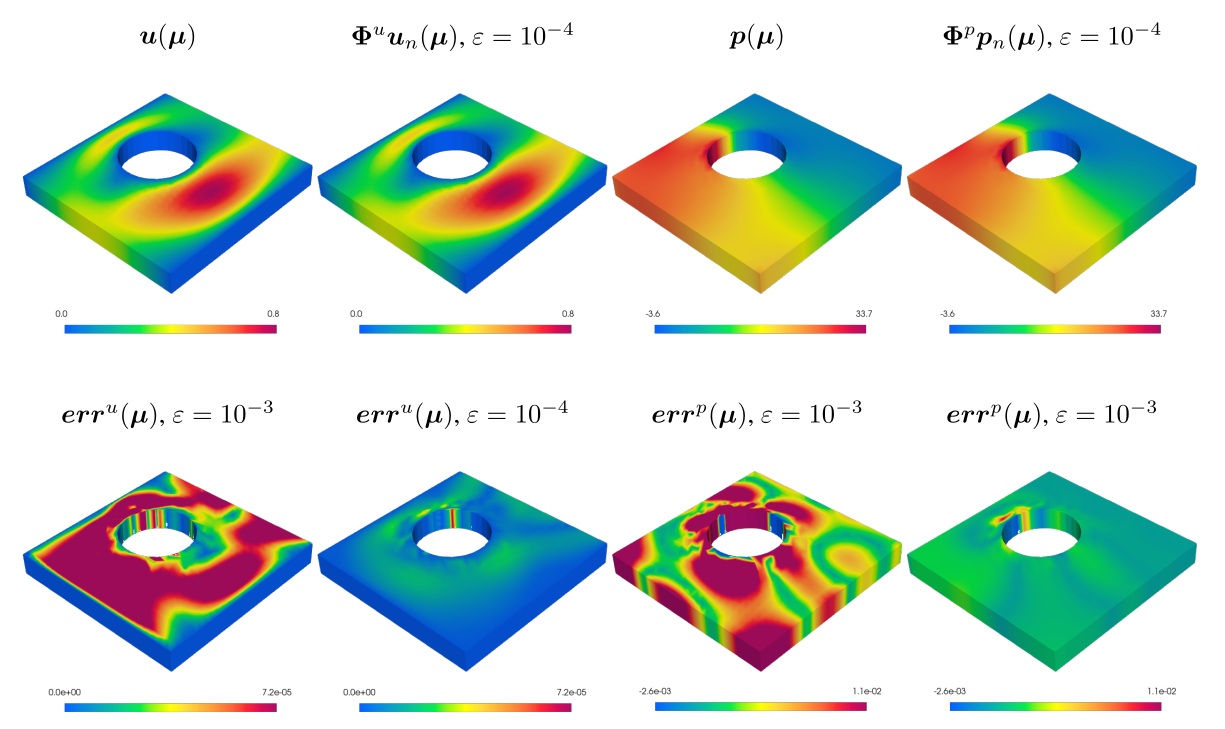
Standard reduced order models assume the mesh stays fixed, which breaks the moment the domain's shape becomes a parameter itself. Combining unfitted finite elements with a mapping back to a reference domain avoids remeshing every time the geometry changes, while keeping the reduced solution close to the full-order one, down to pointwise errors on the order of 10-3–10-4 even near the hole boundary, where the geometry variation is largest.

Unfitted Stokes results on a parameterised domain with a hole

Full-order vs. reduced-order velocity and pressure fields on a square domain with a parameterised circular hole, and the corresponding pointwise errors at two different accuracy levels.

Haemodynamics

Space-time reduced-order models for haemodynamic simulations in patient-specific arteries

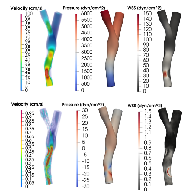
This is the first space-time reduced basis method built specifically for haemodynamics: the physics describing how blood flows through the body over time. The reduced-order model efficiently and accurately reconstructs the full-order velocity, pressure, and wall shear stress fields, on different patient-specific vessels.

Reduced-order velocity, pressure, and wall shear stress fields on a vessel bifurcation, with the corresponding errors

Velocity, pressure, and wall shear stress on a vessel bifurcation. Top row: values reconstructed by the reduced-order model. Bottom row: the corresponding error against the full-order (FEM) solution.

Data assimilation

Finding the hidden Reynolds number of a turbulent flow

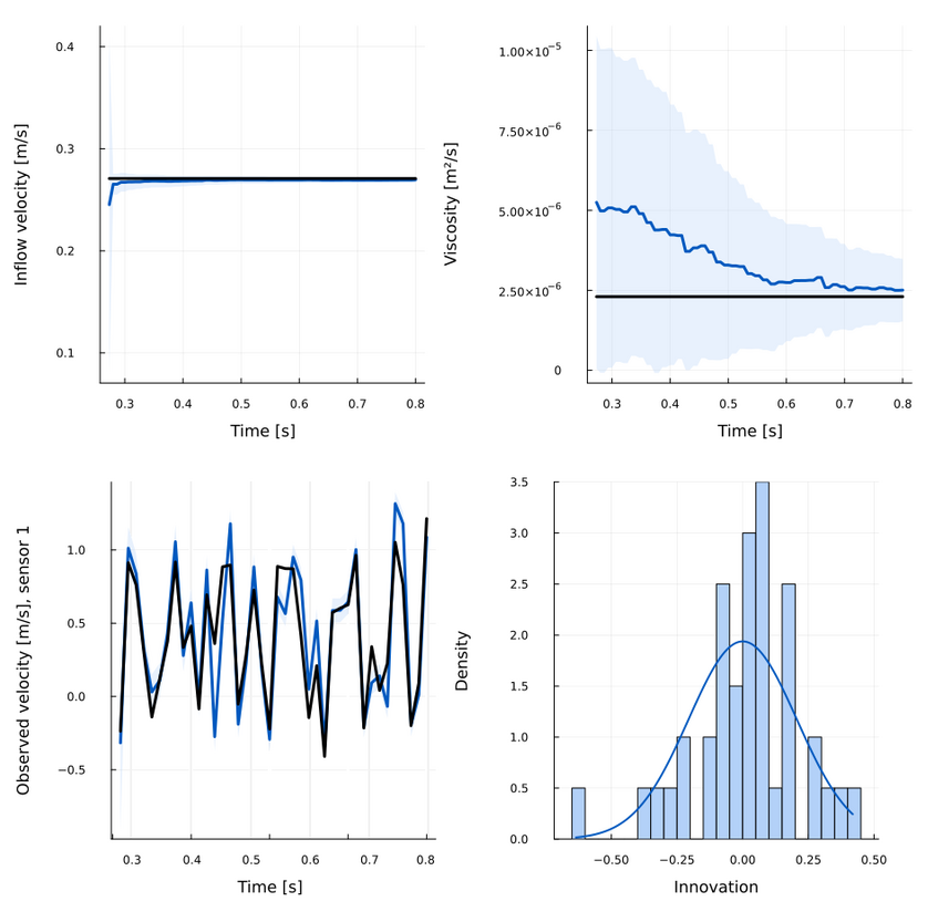
An ensemble Kalman filter recovers the inflow velocity and viscosity of a turbulent Navier-Stokes flow (~6500 DOFs) from sparse, noisy sensors, without ever being told the Reynolds number directly. The innovation statistics check out too: they come out about as Gaussian as the filter assumes, which is the sign that its underlying assumptions actually hold for this problem.

Reynolds number discovery in a turbulent flow

Ensemble Kalman filter estimates for a turbulent Navier-Stokes flow. Top row: inflow velocity and viscosity. Bottom row: a sensor observation and the resulting innovation density.

Data assimilation

Constructing a filter aware of sensor bias

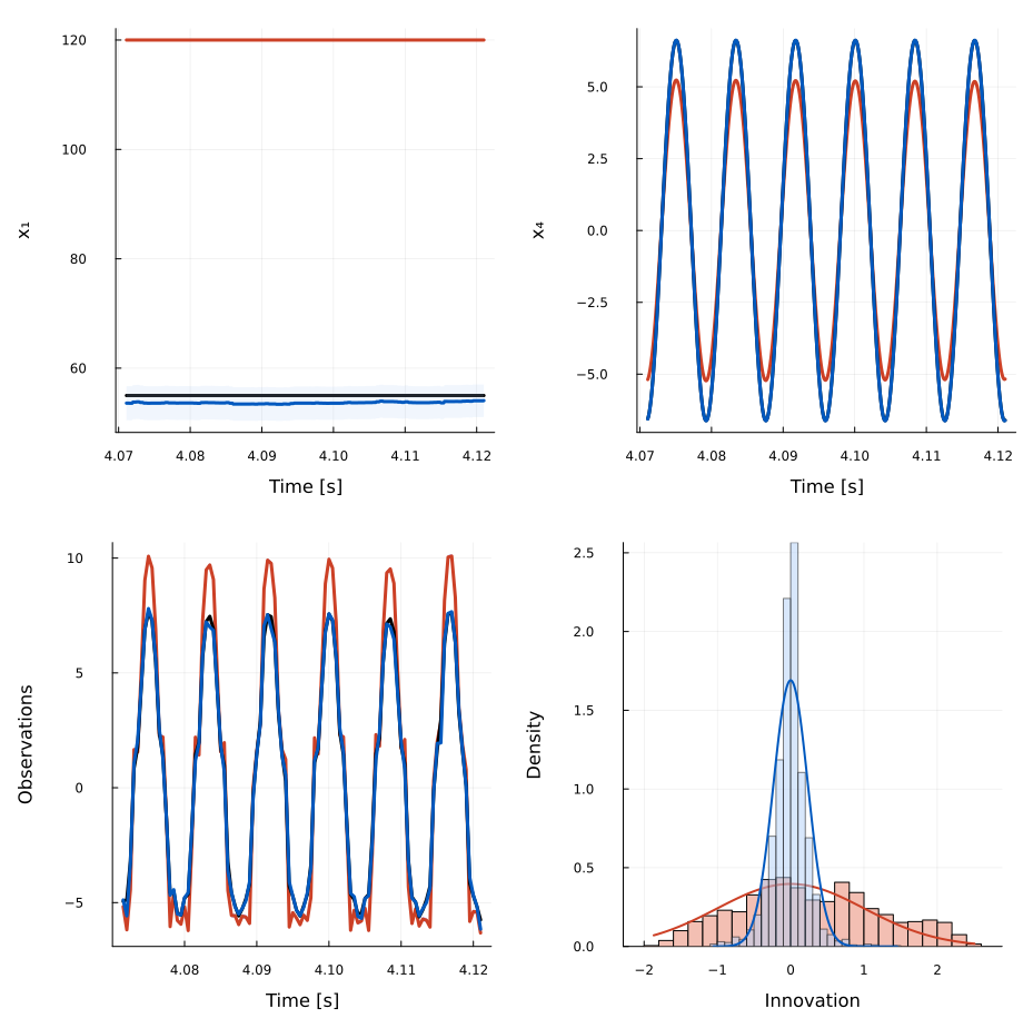
Here the sensor on a Van der Pol oscillator reports a biased version of the true state, not just a noisy one. A Kalman-type filter assumes the innovation, observation minus prediction, is zero-mean Gaussian, and a biased sensor breaks that outright: the bias-unaware filter above converges to a self-consistent but wrong periodic solution. Adding an echo-state network to model the bias itself, re-evaluated as new data arrives, fixes this directly. The bias-aware filter recovers the true state and parameters, and the innovation becomes the Gaussian distribution the filter was assuming all along.

Bias-aware EnKF on a Van der Pol oscillator with a biased sensor

True (black) vs. bias-unaware EnKF (red) vs. bias-aware EnKF (blue). Top row: an estimated parameter (x1) and state (x4). Bottom row: the reconstructed observation and the innovation density each filter produces.

Reservoir computing

A reservoir-computing module that beats ReservoirComputing.jl

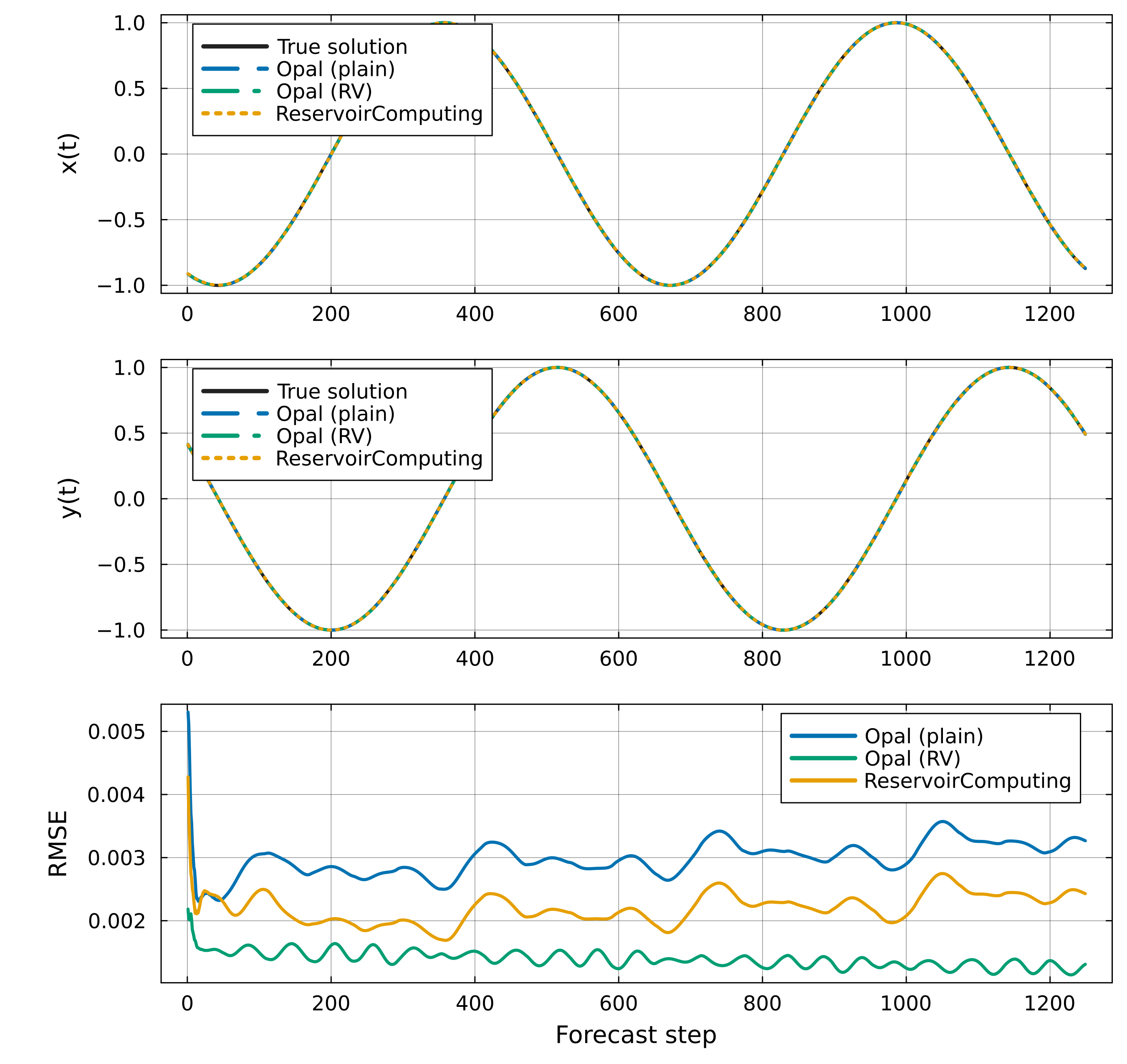
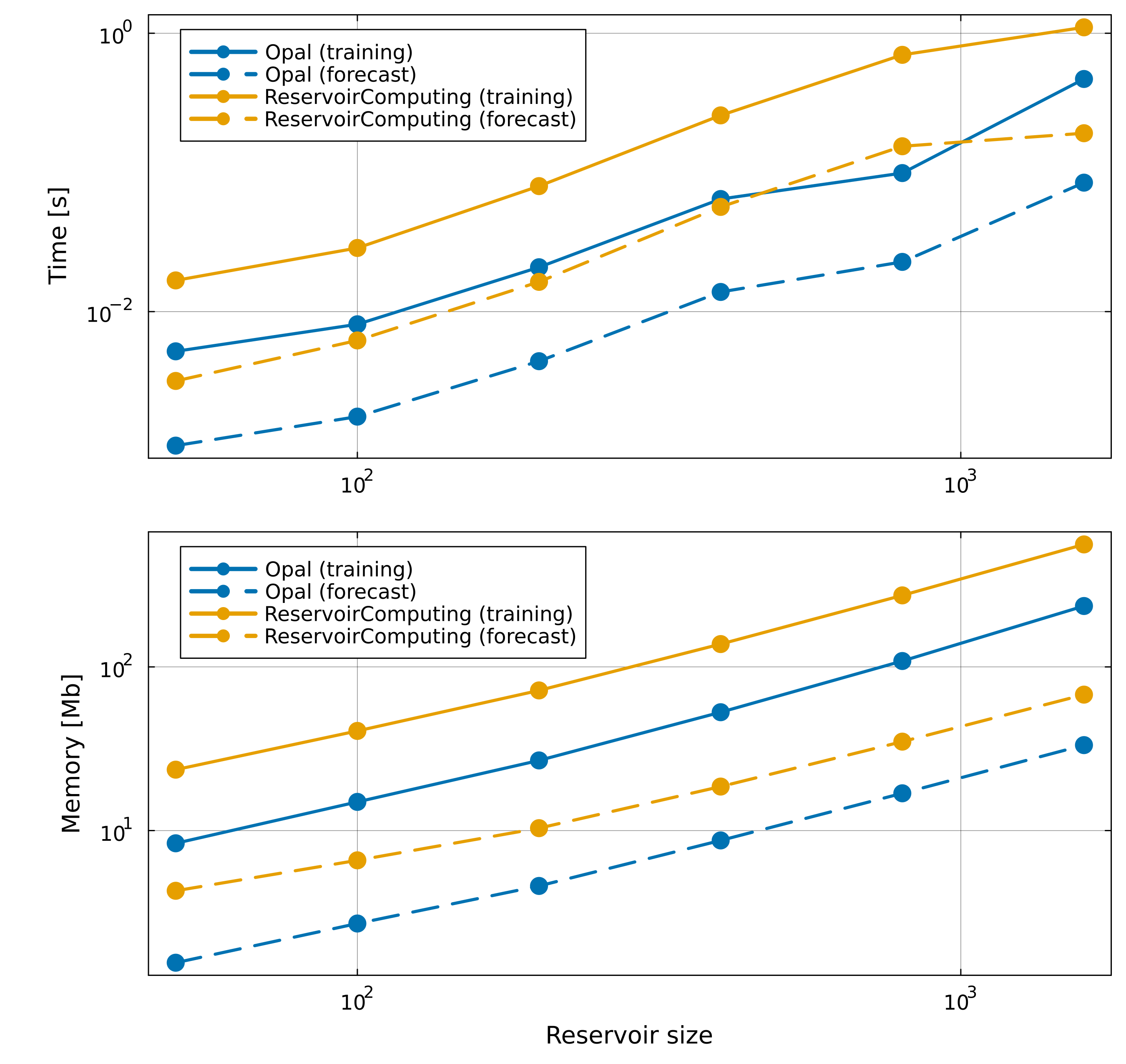
Wrote the echo-state network used for Opal.jl's bias correction from scratch instead of depending on ReservoirComputing.jl, the standard Julia library for reservoir computing. With recycle-validation training it comes out both more accurate and cheaper to train and forecast, across every reservoir size tested.

Reservoir computing accuracy comparison

Forecasting the Hopf bifurcation system over 1250 forecast steps: Opal.jl's echo-state network, plain and with recycle-validation (RV) training, vs. ReservoirComputing.jl.

Reservoir computing training and forecast efficiency comparison

Training and forecast time and memory vs. reservoir size, log-log scale, Opal.jl vs. ReservoirComputing.jl.